Usually, to measure the characteristic curve of a component, a Source Measure Unit (SMU) is needed, which sources a voltage and measures the current it provides with great accuracy. A similar task can be done with a power supply, together with a multimeter to have better accuracy. What is important about those measurements is automation. SMUs can be easily automated through scripts (TSP scripts for example for the Keithley SMUs) and can generate the characteristic curve autonomously, by sourcing different voltages/current and measuring the results.
To conduct similar tests with equipment of different manufacturers, a master controller is needed. With the use of LXI (LAN eXtensions for Instrumentation), this can be done with a computer as the master, commanding the test equipment and logging the results. MATLAB can be used to control the test equipment, log the results and present them in graphs.
All of the LXI compatible equipment use an Ethernet port, the easiest way is to connect them directly to the router, so that they are available to all of the other machines in the network. However, if the router is not close to the test equipment, a raspberry pi can be used to bridge the wireless network with the ethernet network, if all of the test equipment are connected to the raspberry pi. The lnxrouter can be used to setup the connection of the two networks. The routing table on the router or on the controller machine needs to be updated as well.
MATLAB does have an Instrument Control toolbox with some test equipment libraries, but I selected to write my own libraries for the power supply that I am using (Aim TTI MX100TP) and the multimeter (Keithley DMM6500). All of the functions I wrote for the LXI test equipment can be found in the github page. From MATLAB, the procedure is common to any other communication. The connection is opened, and the user writes to the device with an fprintf function call, and gets from the device with a query function call.
A simple example to control the power supply and log measurements from the power supply, as well as from the multimeter. The power supply has overcurrent and overvoltage protection, which can be set manually in the instrument to ensure that an erroneous code would not supply more than the load would handle. A loop is formed which increases the power supply output voltage by 0.2V step on every iteration and gets the voltage measurement from the power supply as well as the current measurement from the multimeter. The measurements are logged and plotted in real time. The multimeter is setup to get 10 measurements and report back the average.
%%% Defines %%%%
clear all;
MX100TP_ip = '192.168.3.107';
DMM6500_ip = '192.168.3.15';
CurrentLimit = 0.5;


% Connect to MX100TP %
MX100TP = instrfind('Type', 'tcpip', 'RemoteHost', MX100TP_ip, 'RemotePort', 9221, 'Tag', '');

if isempty(MX100TP)
    MX100TP = tcpip(MX100TP_ip, 9221);
else
    fclose(MX100TP);
    MX100TP = MX100TP(1);
end
fopen(MX100TP);

% Connect to DMM6500%
DMM6500 = instrfind('Type', 'tcpip', 'RemoteHost', DMM6500_ip, 'RemotePort', 9221, 'Tag', '');
if isempty(DMM6500)
    DMM6500 = tcpip(DMM6500_ip, 5025);
else
    fclose(DMM6500);
    DMM6500 = DMM6500(1);
end
fopen(DMM6500);

%%%%% Setup DMM6500 %%%%%%
DMM6500_Setup(DMM6500, 'FUNC_DC_CURRENT', 1, 10, 10);
%%%%%%% End of Setup %%%%%

voltage = 0;
current_MX100 = 0;
current_DMM6500 = 0;

%%%%%%%%%%%%
disp('Start of Measurements');
M100TP_SetOutputValues(MX100TP, 1, 0, CurrentLimit); % Set current limit for Channel 1
M100TP_SetOutput(MX100TP,1,'ON');

close all;
figure();
f1 = subplot(2,1,1);
h1 = plot(voltage,current_MX100, '-o');
hold on;
h2 = plot(voltage,current_DMM6500, '-*');
xlabel('Voltage [V]'); ylabel('Current [mA]'); grid on; legend('MX100 Current','DMM6500 Current', 'location', 'southeast');
f2 = subplot(2,1,2);
h3 = plot(voltage,voltage*current_MX100, '-o');
hold on;
h4 = plot(voltage,voltage*current_DMM6500, '-*');
xlabel('Voltage [V]'); ylabel('Power [mW]'); grid on; legend('MX100 Power','DMM6500 Power', 'location', 'southeast');

for Voltage=0:0.2:35
    M100TP_SetOutputVoltage(MX100TP, 1, Voltage);
    fprintf('Voltage setpoint: %.1fV\n', Voltage);
    MilliPause(100);
    measvoltage = MX100TP_GetVoltage(MX100TP, 1);
    meascurrent_MX100 = MX100TP_GetCurrent(MX100TP, 1);
    meascurrent_DMM6500 = DMM6500_Read(DMM6500);
    voltage = [voltage measvoltage];
    current_MX100 = [current_MX100 meascurrent_MX100];
    current_DMM6500 = [current_DMM6500 meascurrent_DMM6500];
    set(h1, 'XData', voltage);
    set(h1, 'YData', current_MX100*1000);
    set(h2, 'XData', voltage);
    set(h2, 'YData', current_DMM6500*1000);
    set(h3, 'XData', voltage);
    set(h3, 'YData', voltage.*current_MX100*1000);
    set(h4, 'XData', voltage);
    set(h4, 'YData', voltage.*current_DMM6500*1000);
    drawnow;
end

disp('End of Measurements');
M100TP_SetOutputValues(MX100TP, 1, 0, 0);
M100TP_SetAllOutputs(MX100TP,'OFF');
fclose(MX100TP);
fclose(DMM6500);
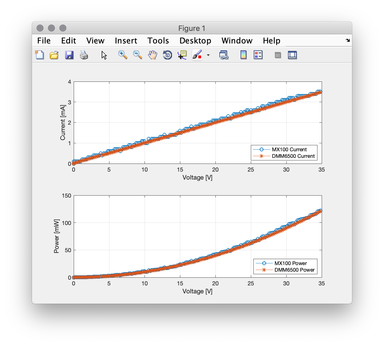
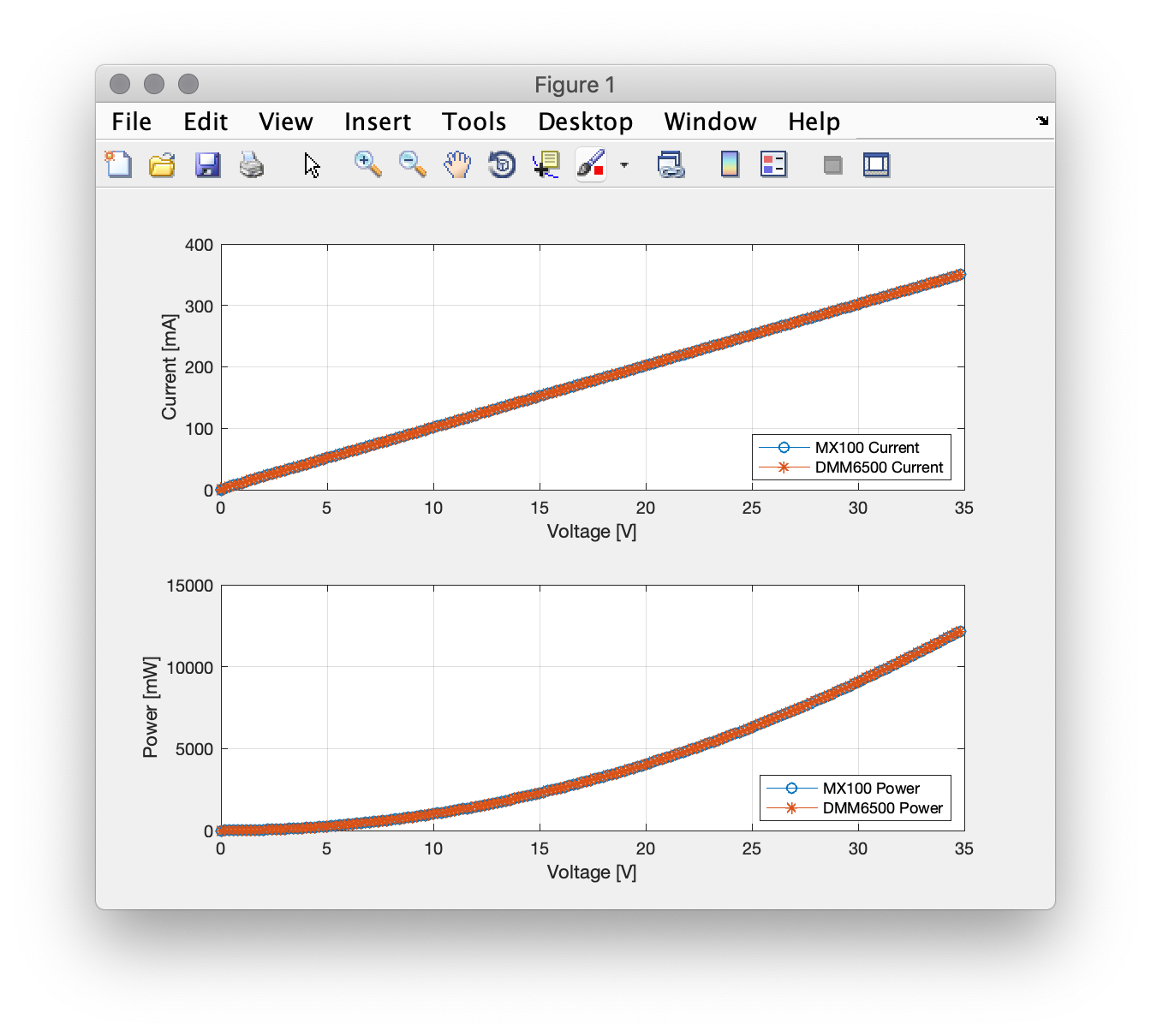
I used the code above to measure two resistors. One was a 100R resistor with the result shown below. As expected, the characteristic is linear.
The second resistor was a 10k one. Because of the much smaller current, the quantization error on the current measurement of the power supply is evident. Even if it has a 0.1mA resolution, still this is not enough. Whereas with the multimetre which has 6.5digits and a 10mA scale, the quantization noise is significantly lower.